Visualizing BEAST 2 time trees

Starting point: strap

The geoscalePhylo() function from the strap package (Bell & Lloyd 2014) is well-known and widely used. It plots a time tree against a nice colorful timescale (the colors are the official color codes of the Commission for the Geological Map of the World), and includes other niceties inherited from plot.phylo(), such as automatically stripping tip names of underscores and printing them in italics. One of the cool options we have at our disposal with geoscalePhylo() is to visualize the uncertainty in the ages of not just the internal nodes (we do that further down below), but also the tips. We can do that using an age range table like the one below:

Note: As pointed out on Facebook by David Bapst, the ages argument of geoscalePhylo() serves primarily for visualizing taxon durations in the fossil record; i.e., the time intervals between the first and last appearance. If a taxon is only known from a single stratigraphically unique occurrence, its first and last appearance will coincide; however, the age uncertainty associated with that occurrence can still be usefully represented using a range. This is what we’re doing below.

age_table <- read.table("~/age_ranges.txt", stringsAsFactors = F)
head(age_table)

##                              V1    V2    V3
## 1         Abrictosaurus_consors 190.8 201.3
## 2       Agilisaurus_louderbacki 163.5 170.3
## 3 Albalophosaurus_yamaguchiorum 132.9 139.8
## 4           Aquilops_americanus  99.6 109.0
## 5       Archaeoceratops_oshimai 113.0 129.4
## 6        Auroraceratops_rugosus 100.5 129.4

We need to reshuffle our age range table a bit, since geoscalePhylo() needs a matrix whose first and last appearance dates are in the right order, and which has exactly the right column and row names:

if(!require("phytools")) {install.packages("phytools")}
if(!require("strap")) {install.packages("strap")}
library(phytools)
library(strap)

my_ages <- cbind(as.numeric(age_table[,3]), as.numeric(age_table[,2]))
colnames(my_ages) <- c("FAD", "LAD")
rownames(my_ages) <- age_table[,1]

tree <- read.nexus("~/my_MCC_tree.tre")

# geoscalePhylo() needs the $root.time element for plotting
tree$root.time <- max(nodeHeights(tree)) + 66.0

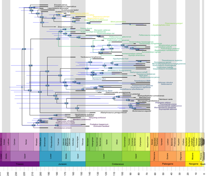
geoscalePhylo(ladderize(tree, right = F), ages = my_ages, x.lim = c(0, 240), cex.tip = 0.7, cex.age = 1.3, cex.ts = 1)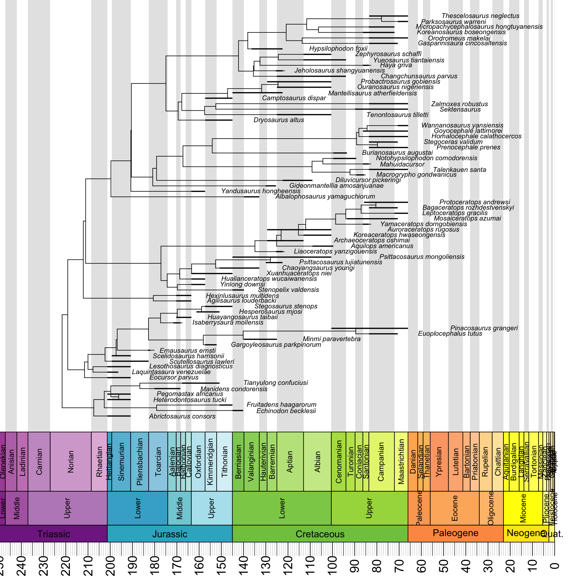

Internally, geoscalePhylo() calls the plot.phylo() function bundled with ape, and so it accepts all of the latter’s arguments. We can make use of this to highlight clades.

Let’s assume that we have a list where each clade to be highlighted gets a pair of “anchors”, whose MRCA is also the MRCA of the entire clade – like this one:

my_dino_list <- list(c("Abrictosaurus_consors", "Tianyulong_confuciusi"),
                     c("Goyocephale_lattimorei", "Wannanosaurus_yansiensis_"),
                     c("Camptosaurus_dispar", "Dryosaurus_altus_"),
                     c("Changchunsaurus_parvus", "Hypsilophodon_foxii_"),
                     c("Aquilops_americanus", "Xuanhuaceratops_niei"),
                     c("Euoplocephalus_tutus", "Gargoyleosaurus_parkpinorum"),
                     c("Hesperosaurus_mjosi", "Isaberrysaura_mollensis"))

What we want to do is (1) find the MRCA of each vector of tip names in the list, (2) assign a certain color to all tips descended from that node, and (3) assign the same color to all branches descended from it. The former is pretty easy:

tip.coloring <- function(tree, clade_list, group_cols) {
  cols <- rep("black", length(tree$tip.label))
  for(i in 1:length(clade_list)) {
    clade_mrca <- getMRCA(tree, clade_list[[i]])
    all_dscndn <- phytools::getDescendants(tree, clade_mrca)
    tips_only <- all_dscndn[all_dscndn <= Ntip(tree)] 
    cols[tips_only] <- group_cols[i]
  }
  return(cols)  
}

Here, we are assuming that the user specifies which color to assign to which clade, rather than creating the colors within the function itself. An additional step is involved when we need to filter the descendant nodes down to tips only: we could get rid of it by using a different function, like Descendants() from phangorn (Schliep 2010), which takes node type as an argument. Here, we exploit the fact that in many of the R packages dealing with phylogenetic trees, the default node labeling scheme assigns numbers from 1 to \(n\) to the tips (leaves), \(n+1\) to the root, and \(n+2\) thru \(2n-1\) to the remaining internal nodes. Conversely, we can count on the fact that nodes labeled with numbers less than or equal to \(n\) are the tips.

The step that consists of coloring all branches descended from the same MRCA is more involved. Fortunately, the indefatigable Liam Revell provides code that does just that in one of the posts on his excellent phytools blog.

Here, we simply package that code into a function analogous to the one shown above:

branch.coloring <- function(tree, clade_list, group_cols) {
  cols <- rep("black", nrow(tree$edge))
  for(i in 1:length(clade_list)) {
    clade_mrca <- getMRCA(tree, clade_list[[i]])
    all_dscndn <- phytools::getDescendants(tree, clade_mrca)
    cols[sapply(all_dscndn, function(x, y) which(y == x), y = tree$edge[,2])] <- group_cols[i]
  }
  return(cols)
}

Adding HPDs: phyloch and weird loops

The next thing we’d like to do than can’t be easily done using any of the many available geoscalePhylo arguments is to add 95% highest posterior density (HPD) intervals to the nodes of our tree.

The first step is to extract the necessary information from the annotated Nexus file produced by TreeAnnotator. There used to be several options for parsing such files; my favorite one was probably read.annotated.nexus() from the OutbreakTools library (Jombart et al. 2014), which unfortunately seems to have lately fallen victim to package dependency troubles. Nevertheless, the read.beast() function from the phyloch package (Heibl 2013) provides a great alternative. Note that we might want to define a new “annotation” (more accurately, add a new element to the list by which the tree is internally represented in R) that doesn’t care about how exactly we got our HPDs (from common ancestor heights? from median heights?) and that can be further manipulated:

if(!require("phyloch")) {
  install.packages("remotes")
  remotes::install_github("fmichonneau/phyloch")
}
library(phyloch)

annot_tree <- phyloch::read.beast("~/my_MCC_tree.tre")

# If the Nexus file has common ancestor node heights in it, extract those; otherwise extract
# the mean/median ones.

if (is.null(annot_tree$`CAheight_95%_HPD_MIN`)) {
  annot_tree$min_ages <- annot_tree$`height_95%_HPD_MIN`
  annot_tree$max_ages <- annot_tree$`height_95%_HPD_MAX`
} else {
  annot_tree$min_ages <- annot_tree$`CAheight_95%_HPD_MIN`
  annot_tree$max_ages <- annot_tree$`CAheight_95%_HPD_MAX`
}

We can also add an arbitrary offset to these ages without overriding the original annotations. Recently, a new class called TreeWOffset was introduced into BEAST 2 to store the age of the youngest tip. This comes in handy when our tree is entirely extinct, and we have age ranges associated with all tips including the youngest one(s). This class allows the ages of such tips to still be sampled from their ranges, effectively leading to the estimation of the “offset” of the tree from the present. Perhaps it is this offset that we want to add to the boundaries of our HPDs. Below, we assume that we have already summarized the posterior of all continuous parameters (including the offset) using LogAnalyser or a similar utility, and printed the results to a parsable text file. The TreeAnnotator-produced Nexus file is of no help here.

params <- read.table("~/loganalyser_params.txt", header = T, stringsAsFactors = F)

# Check whether 'offset' was actually used and logged:

if (length(params$mean[params$statistic == "offset"] != 0)) {
  offset <- params$mean[params$statistic == "offset"]
  annot_tree$min_ages <- annot_tree$min_ages + offset
  annot_tree$max_ages <- annot_tree$max_ages + offset
}

The most complicated step consists of using this info to actually draw the HPDs – this is often done using half-transparent color bars – around the nodes. The basis for what we are going to do is again provided by Liam Revell.

However, as we see below, our attempt to simply reuse the code given in the blog post does not produce satisfying results:

annot_tree$root.time <- max(nodeHeights(annot_tree)) + 66.0
geoscalePhylo(ladderize(annot_tree, right = F), x.lim = c(20, 240), cex.tip = 0.7, cex.age = 1.3, cex.ts = 1)

T1 <- get("last_plot.phylo", envir = .PlotPhyloEnv)

for(i in (Ntip(annot_tree) + 1):(annot_tree$Nnode + Ntip(annot_tree))) {
  lines(x = c(annot_tree$min_ages[i - Ntip(annot_tree)],
              annot_tree$max_ages[i - Ntip(annot_tree)]),
        y = rep(T1$yy[i], 2), lwd = 6, lend = 0,
        col = make.transparent("blue", 0.4))
}

Yes, our HPDs are clearly horrifyingly wide, but they are also not associated with the right nodes – in fact, they are not associated with any nodes, and instead just float freely over the tree. What’s going on here?

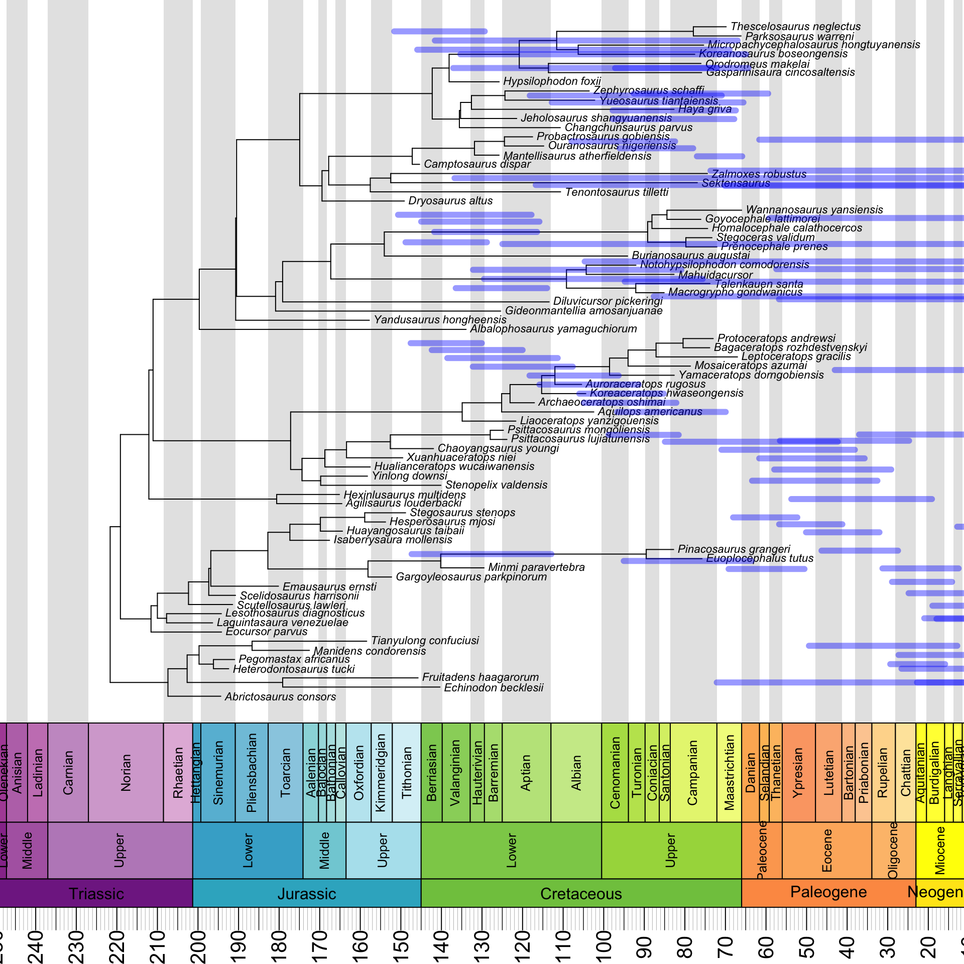
The answer is that the HPDs are reflected about a vertical axis in the middle of the plot. It turns out that we need to subtract both of their endpoints from the root age to fix this:

geoscalePhylo(ladderize(annot_tree, right = F), x.lim = c(20, 240), cex.tip = 0.7, cex.age = 1.3, cex.ts = 1)

T1 <- get("last_plot.phylo", envir = .PlotPhyloEnv)

for(i in (Ntip(annot_tree) + 1):(annot_tree$Nnode + Ntip(annot_tree))) {
  lines(x = c(T1$root.time - annot_tree$min_ages[i - Ntip(annot_tree)],
              T1$root.time - annot_tree$max_ages[i - Ntip(annot_tree)]),
        y = rep(T1$yy[i], 2), lwd = 6, lend = 0,
        col = make.transparent("blue", 0.4))
}

Much better!

Putting it all together

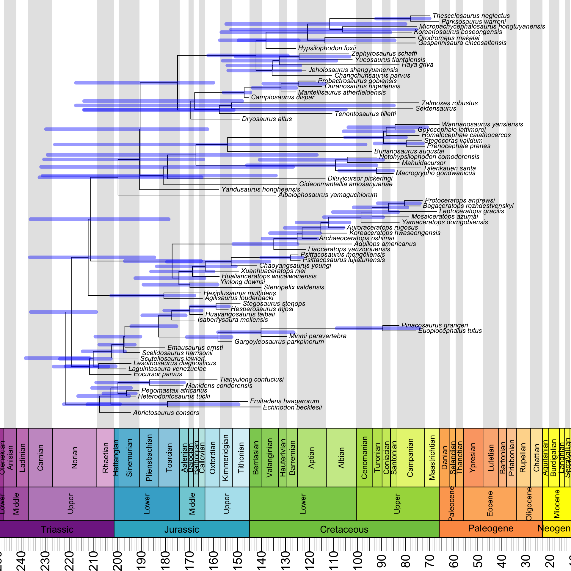
Aside from what we went over above, the function below also parameterizes at what ages to start and stop plotting (so far we’ve been using fixed values for these), automatically draws the right number of colors to highlight clades with from the good-looking viridis palette, and annotates nodes with their posterior probabilities:

if(!require("viridis")) {install.packages("viridis")}
library(viridis)

beast.plotter <- function(basepath, clade_list, xmin, xmax) {
  
  base_tree <- read.nexus(paste(basepath, "my_MCC_tree.tre", sep = ""))
  annot_tree <- phyloch::read.beast(paste(basepath, "my_MCC_tree.tre", sep = ""))
  age_table <- read.table(paste(basepath, "age_ranges.txt", sep = ""), stringsAsFactors = F)
  params <- read.table(paste(basepath, "loganalyser_params.txt", sep = ""),
                       header = T, stringsAsFactors = F)
  
  if (is.null(annot_tree$`CAheight_95%_HPD_MIN`)) {
    annot_tree$min_ages <- annot_tree$`height_95%_HPD_MIN`
    annot_tree$max_ages <- annot_tree$`height_95%_HPD_MAX`
  } else {
    annot_tree$min_ages <- annot_tree$`CAheight_95%_HPD_MIN`
    annot_tree$max_ages <- annot_tree$`CAheight_95%_HPD_MAX`
  }
  
  base_tree$root.time <- max(nodeHeights(base_tree))
  base_tree$node.label <- round(annot_tree$posterior, 2)
  
  if (length(params$mean[params$statistic == "offset"] != 0)) {
    offset <- params$mean[params$statistic == "offset"]
    base_tree$root.time <- base_tree$root.time + offset
    annot_tree$min_ages <- annot_tree$min_ages + offset
    annot_tree$max_ages <- annot_tree$max_ages + offset      
  } else {
    base_tree$root.time <- base_tree$root.time + 66.0
    annot_tree$min_ages <- annot_tree$min_ages + 66.0
    annot_tree$max_ages <- annot_tree$max_ages + 66.0
  }
  
  age_mat <- cbind(as.numeric(age_table[,3]), as.numeric(age_table[,2]))
  rownames(age_mat) <- age_table[,1]
  colnames(age_mat) <- c("FAD", "LAD")
  
  clade_cols <- viridis(length(clade_list), option = "D")
  br_cols <- branch.coloring(ladderize(base_tree, right = F), clade_list, clade_cols)
  tip_cols <- tip.coloring(ladderize(base_tree, right = F), clade_list, clade_cols)

  geoscalePhylo(tree = ladderize(base_tree, right = F), ages = age_mat,
                units = c("Period", "Epoch", "Age"), boxes = "Epoch", cex.tip = 0.7,
                cex.age = 1.3, cex.ts = 1, width = 2, x.lim = c(xmin, xmax),
                edge.color = br_cols, tip.color = tip_cols)
  nodelabels(base_tree$node.label)
  T1 <- get("last_plot.phylo", envir = .PlotPhyloEnv)
  
  # Get shaded bars for the HPD intervals. Credit:
  # http://blog.phytools.org/2017/03/error-bars-on-divergence-times-on.html
  for(i in (Ntip(base_tree) + 1):(base_tree$Nnode + Ntip(base_tree))) {
    lines(x = c(T1$root.time - annot_tree$min_ages[i - Ntip(base_tree)],
                T1$root.time - annot_tree$max_ages[i - Ntip(base_tree)]),
          y = rep(T1$yy[i], 2), lwd = 6, lend = 0,
          col = make.transparent("blue", 0.4))
  }
}

Let’s try it out!

beast.plotter("~/", my_dino_list, 10, 240)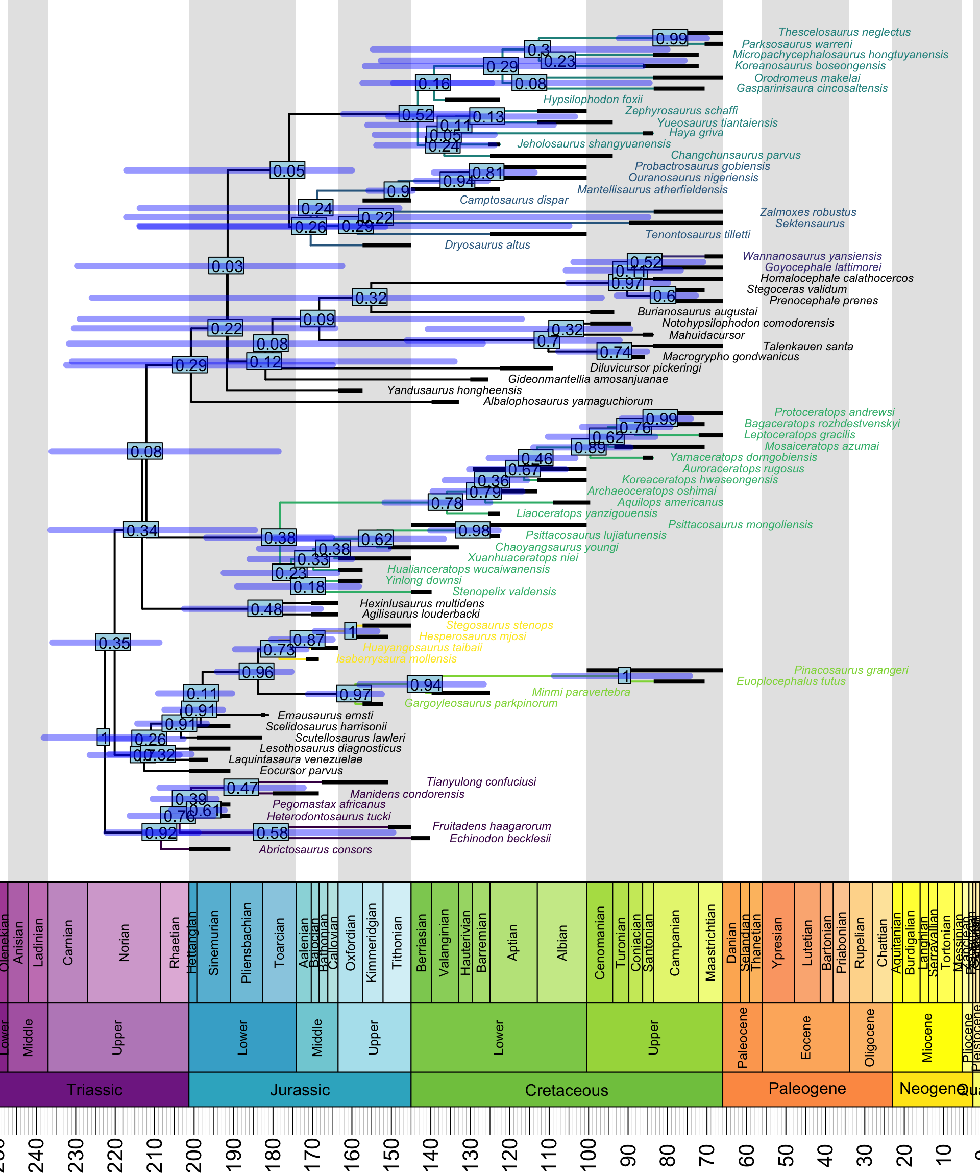

Refs

• Bell MA, Lloyd GT 2014 strap: an R package for plotting phylogenies against stratigraphy and assessing their stratigraphic congruence. Palaeontol 58(2)2: 379–389
• Heibl C 2013 http://www.christophheibl.de/Rpackages.html. Accessed 2020-01-29
• Jombart T, Aanensen DM, Baguelin M, Birrell P, Cauchemez S, Camacho A, Colijn C, Collins C, Cori A, Didelot X, Fraser C, Frost S, Hens N, Hugues J, Höhle M, Opatowski L, Rambaut A, Ratmann O, Soubeyrand S, Suchard MA, Wallinga J, Ypma R, Ferguson N 2014 OutbreakTools: a new platform for disease outbreak analysis using the R software. Epidemics 7: 28–34
• Schliep KP 2010 phangorn: phylogenetic analysis in R. Bioinform 27(4): 592–593